Oceananigans.jl Example: 1D Temperature and Salinity Diffusion at the ice-ocean interface
Date:
This Oceananigans.jl example simulates the diffusion of one-dimensional Gaussian temperature and salinity tracers in an ice-ocean environment.
The governing equations are:
\[\partial_t S + \partial_z ( - \kappa_S \partial_z S) = 0\\ \partial_t T + \partial_z ( - \kappa_T \partial_z T) = 0\]where $\kappa_S$ is the molecular diffusivity of the salt and $\kappa_T$ is the molecular diffusivity of the temperature.
The boundary conditions that simulate the ice-ocean interface are:
- Bottom
- Top
$T_f$ represents the freezing temperature of water, which decreases as salinity increases, a phenomenon known as salt-induced freezing point depression. This effect occurs because dissolved salts interfere with the formation of ice crystals, requiring a lower temperature for the water to solidify.
Here: \(\lambda_1 = -5.73 \times 10^{-2} \quad \text{K}/(\text{g/kg})\\ \lambda_2 = 8.32 \times 10^{-2} \quad \text{K}\\ \lambda_3 = -7.53 \times 10^{-4} \quad \text{K/dbar}\\ Le = \left( \frac{\kappa_T}{\kappa_s} \right) = [1, 100]\\ C_p = 3974 \quad \text{J}/(\text{K} \text{kg})\\ L_f = 3.35 \times 10^5 \quad \text{J}/\text{kg}\\\)
The salinity and temperature follow the initial conditions as: \(T_0(z)=271.0783-1.9217*0.5*(1-\mathbf{erf}(25(z+0.75))\\ S_0(z)=35\) for the domain $z \in [-1, 0]$, which are consistent with the boundary conditions at both the top and bottom. Specifically, at the top $(z = 0)$, the initial temperature and salinity are $T_0(0) = 271.0783$ and $S_0(0) = 35$, while at the bottom $(z = -1)$ are $T_0(-1) = 273$ and $S_0(-1) = 35$.
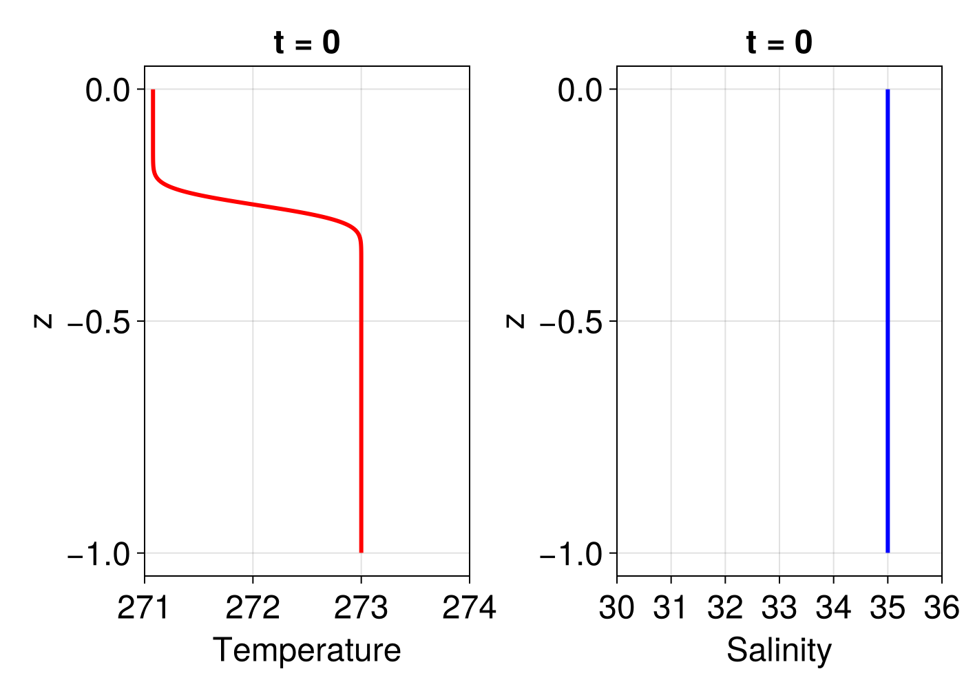
For this example, we set $\text{Le} = 1$, with values of $\kappa_T = 1 \text{m}^2/\text{s}$ and $\kappa_S =0.1 \text{m}^2/\text{s}$. Please note that these values are far from realistic oceanic values of salinity and temperture diffusivities.
The video below illustrates the evolution of both tracers. At the ice-ocean boundary, as the ice melts, salinity decreases near the surface, while the temperature of the surrounding water drops. This happens because the melting process absorbs heat from the water, lowering its temperature—a phenomenon known as latent heat absorption, where the heat is used to convert solid ice into liquid water.
To access the Oceananigans.jl file, please download here!
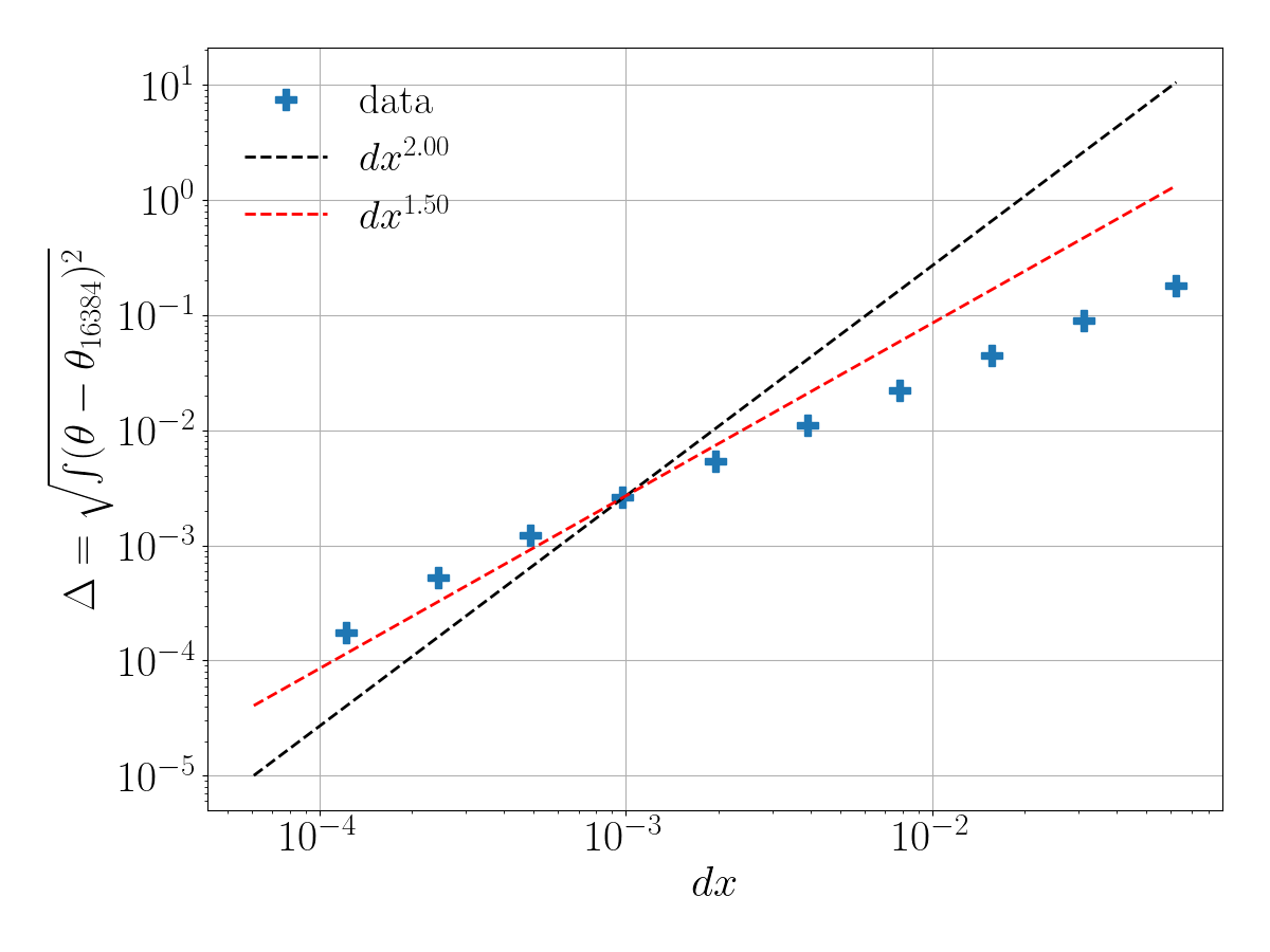
We use this example to compute the relative error from different numerical resolutions. Our ‘theoretical solution’ corresponds to the spatial resolution equal to $16384$. We observe that this scales similarly to $ dx^{1.5}$, which is slightly less than the second-order spatial numerical scheme used in Oceananigans.
Additionally, we compute the evolution of the relative error between the output of our simulation, using a numerical resolution of 1024 grid points, and the predicted values from the boundary equations. Its evolution is shown below,
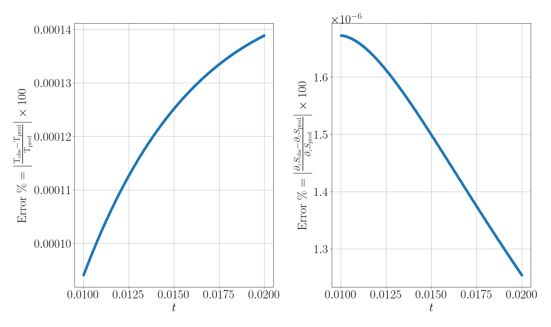
where: \(T_{\text{pred}}=273+\lambda_1 S + \lambda_2\\ T_{\text{obs}}=\frac{T_{n_z}+T_{n_z+1}}{2}\\ \partial_z S_{\text{pred}} = Le \, C_p \, L_f^{-1} \, S \, \partial_z T\\ \partial_z S_{\text{obs}} = \frac{S_{n_z}-S_{n_z+1}}{dz}\)
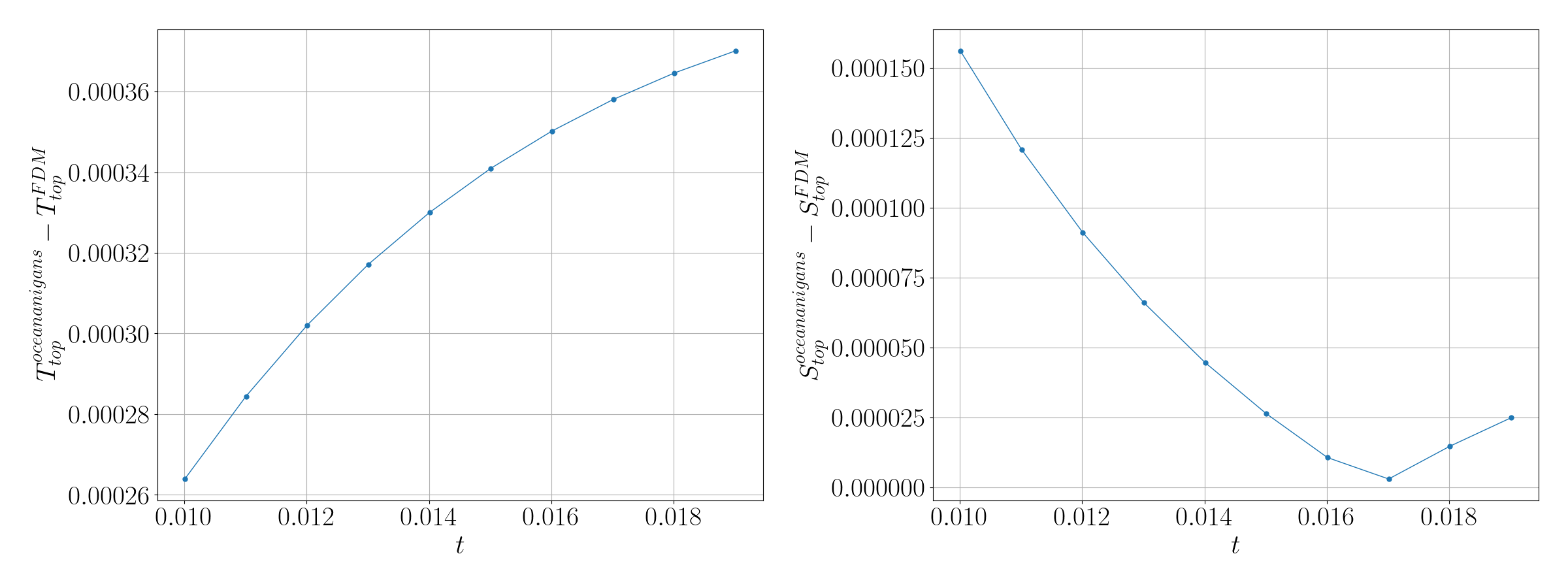
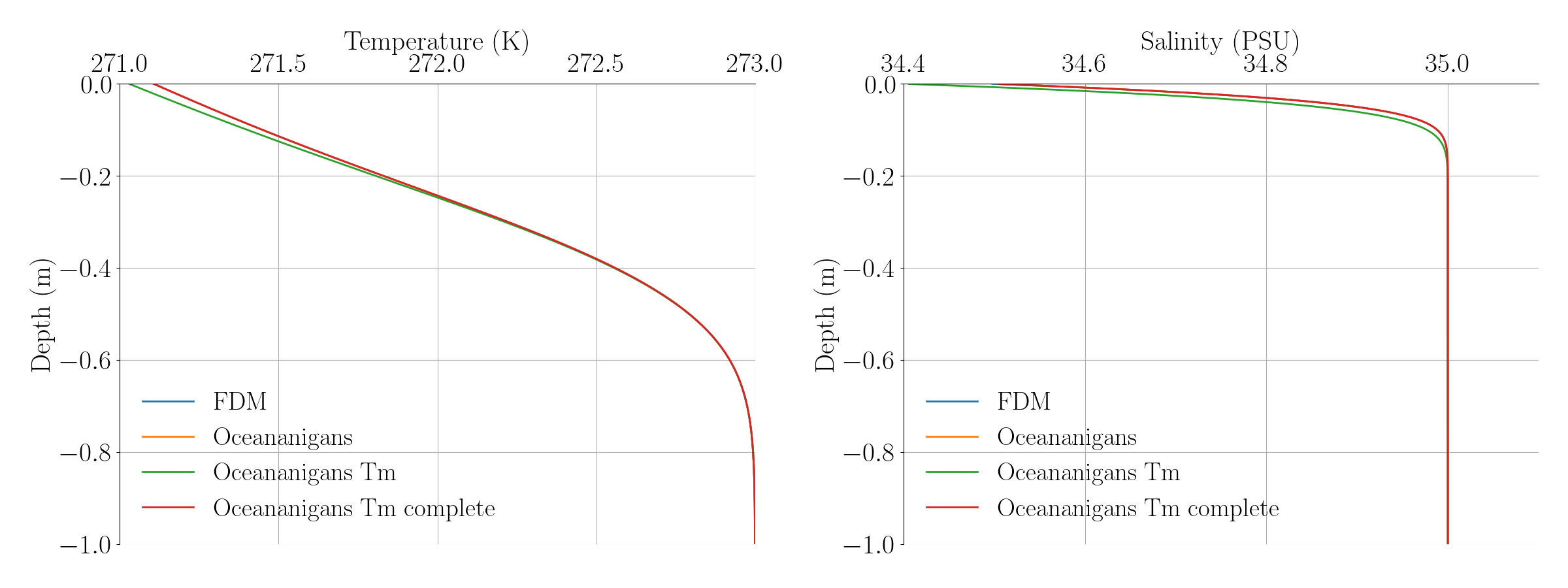
To verify the accuracy of our implementation of the melt boundary condition in Oceananigans, we compare our results with those from a finite difference code written in Fortran. In the Fortran code, we use the same setup with 384 grid points and $\Delta t = 2 \times 10^{-3}$. Our Oceananigans simulation uses 1024 grid points with $\Delta t = 1 \times 10^{-7}$. At the same final time of 0.02, the salinity and temperature profiles are as follows:
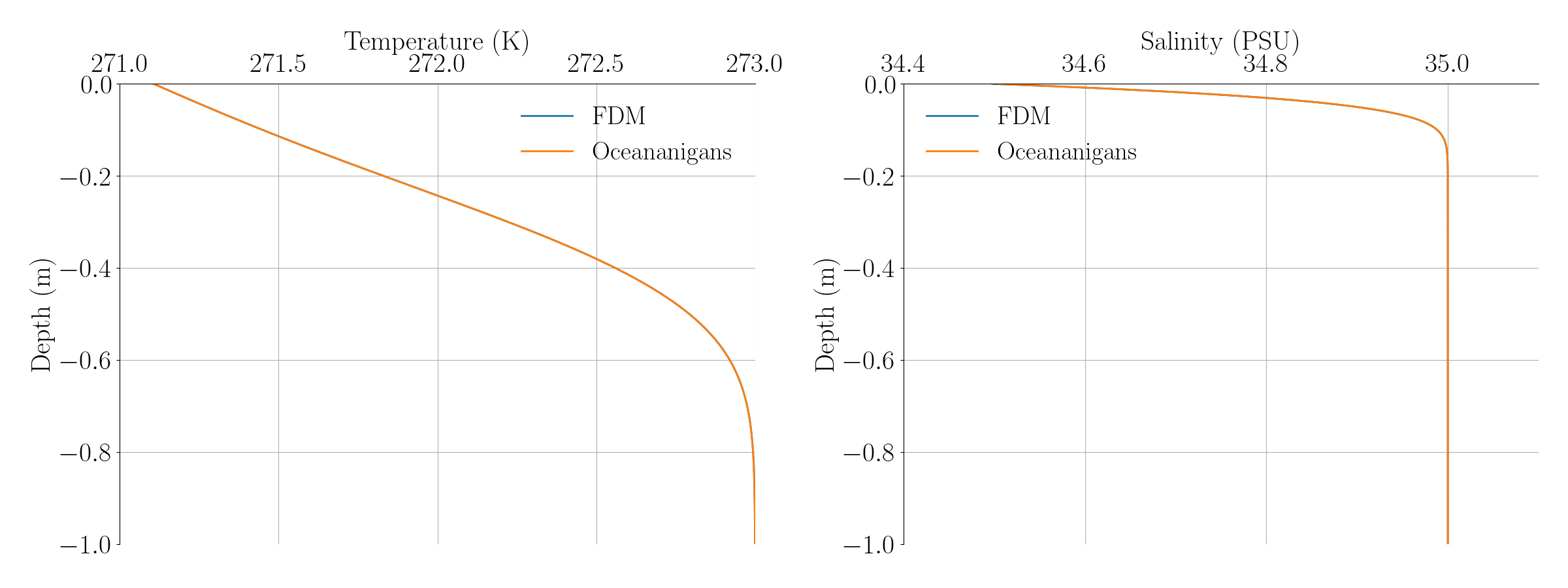
The error between the two models for salinity and temperature at the boundary reaches:
We also implement an alternative approach to include the melt conditions. In the first approximation, we combine the boundary conditions as $ S = (T - 273)/\lambda_1 $ and $ \partial_z S = 1/\alpha S \partial_z T $, with $\alpha=L_f/(Le \, C_p)$, as follows:
\[\frac{S - S_0}{\Delta z} = \frac{1}{\alpha} \frac{S\,(T - T_0)}{\Delta z}\]This leads to the following equation:
\[\alpha \left( \frac{T - 273}{\lambda_1} - S_0 \right) = \frac{(T - 273)(T - T_0)}{\lambda_1}\]which simplifies to:
\[T^2 + T(-\alpha - T_0 - 273) + \alpha \lambda_1 S + 273 (T + \alpha) = 0\]In a more complete approximation, using $ S = (T - 273 - \lambda_2)/\lambda_1 $, the second-order equation for the value of $ T $ at the ice-ocean interface becomes:
\[T^2 + T(-\alpha - T_0 - 273 - \lambda_2) + \alpha \lambda_1 S + (273 + \lambda_2)(T + \alpha) = 0\]We compare the four models at the same final time of 0.02. “Oceananigans T” represents the first approximation, while “Oceananigans T complete” represents the second one. We observe that the “Oceananigans T” model displays the largest discrepancies compared to the other models, indicating that neglecting $\lambda_2$ leads to unrealistic values of salinity and temperature.
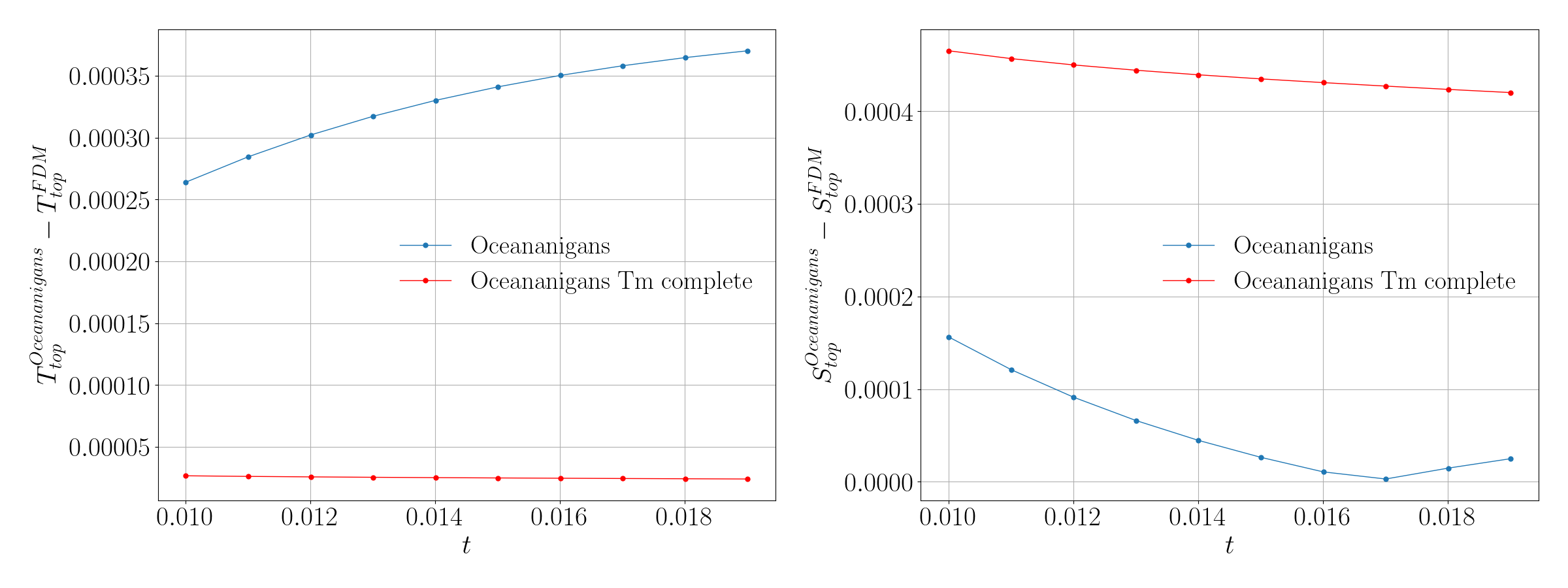
Comparing the error between the first Oceananigans implementation and the FFM model with the error from the quadratic equation implementation and the FFM model, we observe an increase in the error in particular in the temperature, as shown in the figure below.
To access the alternative version of the boundary condition implementation, please download here!
