Oceananigans.jl Example: 1D Temperature and Salinity Diffusion
Date:
This Oceananigans.jl example simulates the diffusion of a one-dimensional Gaussian temperature and salinity tracers.
The governing equations are:
\[\partial_t S + \partial_z ( - \kappa_S \partial_z S) = 0\\ \partial_t T + \partial_z ( - \kappa_T \partial_z T) = 0\]where $\kappa_S$ is the molecular diffusivity of the salt and $\kappa_T$ is the molecular diffusivity of the temperature.
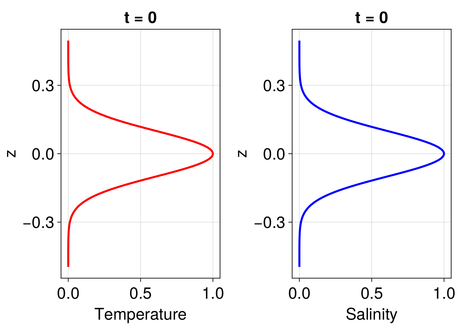
Our objective is to observe the temperature and salinity diffusion of a Gaussian function. The salinity and temperature follow the initial conditions as: $exp(-z^2 / (\sigma^2))$ where $\sigma=0.2$. The figure below shows these initial conditions.

Next, we set up the molecular diffusivity for salt and temperature. In the ocean, the scalar diffusivity of temperature is 2 orders of magnitude larger than that of salt, with values of $\kappa_S \approx 10^{-9} \, \text{m}^2/\text{s}$ and $\kappa_T \approx 10^{-7} \, \text{m}^2/\text{s}$. This leads to a Lewis number of approximately 100. The Lewis number is defined as $\text{Le} = \frac{\text{Sc}}{\text{Pr}}$, where $\text{Sc} = \frac{\nu}{\kappa_S}$ is the Schmidt number and $\text{Pr} = \frac{\nu}{\kappa_T}$ is the Prandtl number.
For this example, we choose $\text{Le} =10$, with unrealistically high molecular viscosities in order to observe only the rate difference between them. The video below displays the evolution of both tracers. As expected, the temperature diffuses faster than the salinity.
To access the Oceananigans.jl file, please download here!
